Linux kernel for GPU Workload

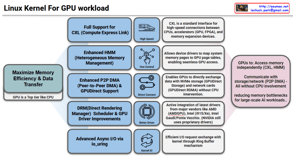
Linux Kernel GPU Workload Support Features

Goal: Maximize Memory Efficiency & Data Transfer

The core objective is to treat GPUs as a top-tier component like CPUs, reducing memory bottlenecks for large-scale AI workloads.

Key Features

1. Full CXL (Compute Express Link) Support

  • Standard interface for high-speed connections between CPUs, accelerators (GPU, FPGA), and memory expansion devices
  • Enables high-speed data transfer

2. Enhanced HMM (Heterogeneous Memory Management)

  • Heterogeneous memory management capabilities
  • Allows device drivers to map system memory pages to GPU page tables
  • Enables seamless GPU memory access

3. Enhanced P2P DMA & GPUDirect Support

  • Enables direct data exchange between GPUs
  • Direct communication with NVMe storage and network cards (GPUDirect RDMA)
  • Operates without CPU intervention for improved performance

4. DRM Scheduler & GPU Driver Improvements

  • Enhanced Direct Rendering Manager scheduling functionality
  • Active integration of latest drivers from major vendors: AMD (AMDGPU), Intel (i915/Xe), Intel Gaudi/Ponte Vecchio
  • NVIDIA still uses proprietary drivers

5. Advanced Async I/O via io_uring

  • Efficient I/O request exchange with kernel through Ring Buffer mechanism
  • Optimized asynchronous I/O performance

Summary

The Linux kernel now enables GPUs to independently access memory (CXL, HMM), storage, and network resources (P2P DMA, GPUDirect) without CPU involvement. Enhanced drivers from AMD, Intel, and improved schedulers optimize GPU workload management. These features collectively eliminate CPU bottlenecks, making the kernel highly efficient for large-scale AI and HPC workloads.

#LinuxKernel #GPU #AI #HPC #CXL #HMM #GPUDirect #P2PDMA #AMDGPU #IntelGPU #MachineLearning #HighPerformanceComputing #DRM #io_uring #HeterogeneousComputing #DataCenter #CloudComputing

With Claude

FP8 Mixed-Precision Training

FP8 Mixed-Precision Training Interpretation

This image is a technical diagram showing FP8 (8-bit Floating Point) Mixed-Precision Training methodology.

Three Main Architectures

1. Mixture of Experts (MoE)

  • Input: Starts with BF16 precision
  • Calc (1): Router output & input hidden states → BF16
  • Calc (2): Expert FFN (Feed-Forward Network) → FP8 computation
  • Calc (3): Accumulation → FP32
  • Transmit (Dispatch): Token dispatch (All-to-All) → FP8
  • Transmit (Combine): Combine expert outputs → BF16
  • Output: BF16

2. Multi-head Latent Attention

  • Input: BF16
  • Calc (1): Input hidden states → BF16
  • Calc (2): Projection/Query/Key/Value → FP8
  • Calc (3): Key/Value compression → BF16
  • Stabilization: RMSNorm → FP32
  • Output: Output hidden states → BF16

3. Multi-Token Prediction

  • Input: BF16
  • Calc (1): Embedding layer output → BF16
  • Calc (2): Transformer block → FP8
  • Calc (3): RMSNorm → FP32
  • Calc (4): Linear projection → BF16
  • Output: Output hidden states → BF16

Precision Strategy (Bottom Boxes)

🟦 BF16 (Default)

  • Works for most tasks
  • Balanced speed/stability

🟪 BF8 (Fastest)

  • For large compute/data movement
  • Very energy-efficient

🟣 BF32 (Safest/Most Precise)

  • For accuracy-critical or sensitive math operations

Summary

FP8 mixed-precision training strategically uses different numerical precisions across model operations: FP8 for compute-intensive operations (FFN, attention, transformers) to maximize speed and efficiency, FP32 for sensitive operations like accumulation and normalization to maintain numerical stability, and BF16 for input/output and communication to balance performance. This approach enables faster training with lower energy consumption while preserving model accuracy, making it ideal for training large-scale AI models efficiently.


#FP8Training #MixedPrecision #AIOptimization #DeepLearning #ModelEfficiency #NeuralNetworks #ComputeOptimization #MLPerformance #TransformerTraining #EfficientAI #LowPrecisionTraining #AIInfrastructure #MachineLearning #GPUOptimization #ModelTraining

With Claude

LLM goes with Computing-Power-Cooling

LLM’s Computing-Power-Cooling Relationship

This diagram illustrates the technical architecture and potential issues that can occur when operating LLMs (Large Language Models).

Normal Operation (Top Left)

  1. Computing Requires – LLM workload is delivered to the processor
  2. Power Requires – Power supplied via DVFS (Dynamic Voltage and Frequency Scaling)
  3. Heat Generated – Heat is produced during computing processes
  4. Cooling Requires – Temperature management through proper cooling systems

Problem Scenarios

Power Issue (Top Right)

  • Symptom: Insufficient power (kW & Quality)
  • Results:
    • Computing performance degradation
    • Power throttling or errors
    • LLM workload errors

Cooling Issue (Bottom Right)

  • Symptom: Insufficient cooling (Temperature & Density)
  • Results:
    • Abnormal heat generation
    • Thermal throttling or errors
    • Computing performance degradation
    • LLM workload errors

Key Message

For stable LLM operations, the three elements of Computing-Power-Cooling must be balanced. If any one element is insufficient, it leads to system-wide performance degradation or errors. This emphasizes that AI infrastructure design must consider not only computing power but also adequate power supply and cooling systems together.


Summary

  • LLM operation requires a critical balance between computing, power supply, and cooling infrastructure.
  • Insufficient power causes power throttling, while inadequate cooling leads to thermal throttling, both resulting in workload errors.
  • Successful AI infrastructure design must holistically address all three components rather than focusing solely on computational capacity.

#LLM #AIInfrastructure #DataCenter #ThermalManagement #PowerManagement #AIOperations #MachineLearning #HPC #DataCenterCooling #AIHardware #ComputeOptimization #MLOps #TechInfrastructure #AIatScale #GreenAI

WIth Claude

Basic LLM Workflow

Basic LLM Workflow Interpretation

This diagram illustrates how data flows through various hardware components during the inference process of a Large Language Model (LLM).

Step-by-Step Breakdown

① Initialization Phase (Warm weights)

  • Model weights are loaded from SSD → DRAM → HBM (High Bandwidth Memory)
  • Weights are distributed and shared across multiple GPUs

② Input Processing (CPU tokenizes/batches)

  • CPU tokenizes input text and processes batches
  • Data is transferred through DRAM buffer to GPU

③ GPU Inference Execution

  • GPU performs Attention and FFN (Feed-Forward Network) computations from HBM
  • KV cache (Key-Value cache) is stored in HBM
  • If HBM is tight, KV cache can be offloaded to DRAM or SSD

④ Distributed Communication (NvLink/Infiniband)

  • Intra-node: High-speed communication between GPUs via NvLink (with NVSwitch if available)
  • Inter-node: Parallel communication through InfiniBand or NCCL

⑤ Post-processing (CPU decoding/post)

  • CPU decodes generated tokens and performs post-processing
  • Logs and caches are saved to SSD

Key Characteristics

This architecture leverages a memory hierarchy to efficiently execute large-scale models:

  • SSD: Long-term storage (slowest, largest capacity)
  • DRAM: Intermediate buffer
  • HBM: GPU-dedicated high-speed memory (fastest, limited capacity)

When model size exceeds GPU memory, strategies include distributing across multiple GPUs or offloading data to higher-level memory tiers.


Summary

This diagram shows how LLMs process data through a memory hierarchy (SSD→DRAM→HBM) across CPU and GPU components. The workflow involves loading model weights, tokenizing inputs on CPU, running inference on GPU with HBM, and using distributed communication (NvLink/InfiniBand) for multi-GPU setups. Memory management strategies like KV cache offloading enable efficient execution of large models that exceed single GPU capacity.

#LLM #DeepLearning #GPUComputing #MachineLearning #AIInfrastructure #NeuralNetworks #DistributedComputing #HPC #ModelOptimization #AIArchitecture #NvLink #Transformer #MLOps #AIEngineering #ComputerArchitecture

With Claude

The Perfect Paradox

The Perfect Paradox – Analysis

This diagram illustrates “The Perfect Paradox”, explaining the relationship between effort and results. Here are the key concepts:

Graph Analysis

Axes:

  • X-axis: Effort
  • Y-axis: Result

Pattern:

  • Initially, results increase proportionally with effort
  • After the Inflection Point (green circle), dramatically increased effort yields minimal or even diminishing returns
  • “Perfect” exists in an unreachable zone

Core Message

“Good Enough (Satisfying)”

  • Located near the inflection point
  • Represents the optimal effort-to-result ratio

The Central Paradox:

“Before ‘perfect’ lies ‘infinite’.”

This means achieving perfection requires infinite effort.

AI Connection

The bottom arrow shows the evolution of approaches:

  • Rule-based ApproachData-Driven Approach

Key Insight:

“While data-driven AI is now far beyond ‘good enough’, it remains imperfect.”

This suggests that modern AI achieves high performance, but pursuing practical utility is more rational than chasing perfection.


Summary

The Perfect Paradox shows that after a certain inflection point, exponentially more effort produces minimal improvement, making “perfect” practically unreachable. The optimal strategy is achieving “good enough” – the sweet spot where effort and results are balanced. Modern data-driven AI has surpassed “good enough” but remains imperfect, demonstrating that practical excellence trumps impossible perfection.

#PerfectParadox #DiminishingReturns #GoodEnough #EffortVsResults #PracticalExcellence #AILimitations #DataDrivenAI #InflectionPoint #OptimizationStrategy #PerfectionismVsPragmatism #ProductivityInsights #SmartEffort #AIPhilosophy #EfficiencyMatters #RealisticGoals

AI-driven operational intelligence loop

AI-Driven Operational Intelligence Loop


1️⃣ High-Resolution & Accurate Data


Collect precise, high-frequency sensor data across all systems to ensure reliability and synchronization.

2️⃣ Change Detection & Connectivity


Continuously monitor data variations and correlations to identify anomalies and causal relationships in real time.

3️⃣ Analytics & Classification


Analyze detected changes, classify events by impact and severity, and generate actionable insights for optimization.

4️⃣ Response Framework


Define and execute automated or semi-automated response strategies based on analysis and classification results.

5️⃣ AI Application & Continuous Learning


Use AI to automate steps 2–4, enhance prediction accuracy, and continuously improve operations through feedback and model retraining.

Loop Concept
1 Data → 2 Detection → 3 Analysis → 4 Response → 5 AI → (Feedback & Optimization)
Goal:
Build a self-optimizing operational ecosystem that integrates data, AI, and automation for smarter, more reliable digital operations.