
Never happen . But remember
The Computing for the Fair Human Life.
Never happen . But remember


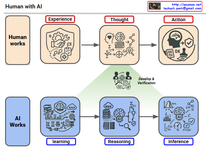
This image titled “Human with AI” illustrates the collaborative structure between humans and AI.
Humans operate through three stages:
AI operates through similar three stages:
The green arrow in the center with “Develop & Verification” represents the process where humans verify AI’s reasoning results and make final judgments (Thought) to connect them to actual actions (Action).
In other words, when AI analyzes data and presents reasoning results, humans review and verify them to ultimately decide whether to execute – representing a Human-in-the-loop system. AI assists decision-making, but the final judgment and action are under human responsibility.
This diagram illustrates a Human-in-the-loop AI system where AI processes data and provides reasoning, but humans retain final decision-making authority. Both humans and AI follow similar learning-thinking-acting cycles, but human verification serves as the critical bridge between AI inference and real-world action. This structure emphasizes responsible AI deployment with human oversight.
#HumanAI #AICollaboration #HumanInTheLoop #AIGovernance #ResponsibleAI #AIDecisionMaking #HumanOversight #AIVerification #HumanCenteredAI #AIEthics
With Claude
Memory
Network
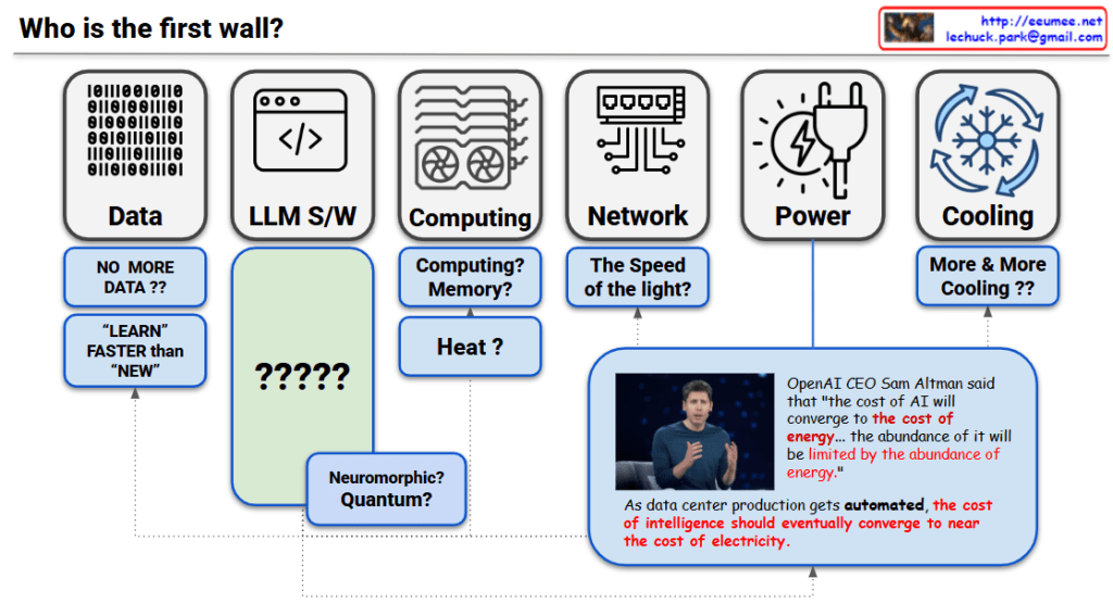
Critical Bottlenecks by Timeline:
The “first wall” in AI scaling is not a single barrier but a multi-layered constraint system that emerges sequentially over time. Today’s immediate challenges are memory bandwidth and data quality, followed by power infrastructure limitations in the mid-term, and ultimately the fundamental physical constraint of the speed of light. As Sam Altman emphasized, AI’s future abundance will be fundamentally limited by energy abundance, with all bottlenecks interconnected through the computing→heat→cooling→power chain.
#AIScaling #AIBottleneck #MemoryBandwidth #HBM #DataCenterPower #AIInfrastructure #SpeedOfLight #SyntheticData #EnergyConstraint #AIFuture #ComputingLimits #GPUCluster #TestTimeCompute #MixtureOfExperts #SamAltman #AIResearch #MachineLearning #DeepLearning #AIHardware #TechInfrastructure
With Claude

This diagram illustrates how data centers are transforming as they enter the AI era.
The top section shows major technology revolutions and their timelines:
Conventional data centers consisted of the following core components:
These were designed as relatively independent layers.
With the introduction of AI (especially LLMs), data centers require specialized infrastructure:
The circular connection in the center of the diagram represents the most critical feature of AI data centers:
Unlike traditional data centers, in AI data centers:
These elements must be closely integrated in design, and optimizing just one element cannot guarantee overall system performance.
AI workloads require moving beyond the traditional layer-by-layer independent design approach of conventional data centers, demanding that computing-network-power-cooling be designed as one integrated system. This demonstrates that a holistic approach is essential when building AI data centers.
AI data centers fundamentally differ from traditional data centers through the tight integration of computing, networking, power, and cooling systems. GPU-based AI workloads create unprecedented power density and heat generation, requiring liquid cooling and HVDC power systems. Success in AI infrastructure demands holistic design where all components are co-optimized rather than independently engineered.
#AIDataCenter #DataCenterEvolution #GPUInfrastructure #LiquidCooling #AIComputing #LLM #DataCenterDesign #HighPerformanceComputing #AIInfrastructure #HVDC #HolisticDesign #CloudComputing #DataCenterCooling #AIWorkloads #FutureOfDataCenters
With Claude

This diagram illustrates the fundamental purpose and stages of optimization.
Input → Processing → Output → Verification
Optimization aims to increase speed and reduce resources by removing unnecessary operations. It follows a staged approach starting from software-level improvements and extending to hardware implementation when needed. The process ensures predictable, verifiable results through deterministic inputs/outputs and rule-based methods.
#Optimization #PerformanceTuning #CodeOptimization #AlgorithmImprovement #SoftwareEngineering #HardwareAcceleration #ResourceManagement #SpeedOptimization #MemoryOptimization #SystemDesign #Benchmarking #Profiling #EfficientCode #ComputerScience #SoftwareDevelopment
With Claude

This image, titled “New For AI,” systematically organizes the essential components required for building AI systems.
Left Domain – Computing Axis (Turquoise)
Right Domain – Infrastructure Axis (Light Blue)
3. Enormous Energy
Large-scale power supply to drive AI computing
Meaning of the Chain Link Icon:
Technologies to enhance AI model performance and efficiency:
Hardware and network technologies enabling massive computation:
Technologies for stable and efficient power supply:
Securing cooling system efficiency and stability:
This diagram emphasizes that for successful AI implementation:
The central link particularly visualizes the interdependent relationship where “increasing computing power requires strengthening energy and cooling in tandem, and computing performance cannot be realized without infrastructure support.”
AI systems require two inseparable pillars: Computing (Data/Chips) and Infrastructure (Power/Cooling), which must be tightly integrated and optimized together like links in a chain. Each pillar is supported by advanced technologies spanning from AI model optimization (FlashAttention, Quantization) to next-gen hardware (GB200, TPU) and sustainable infrastructure (SMR, Liquid Cooling, AI-driven optimization). The key insight is that scaling AI performance demands simultaneous advancement across all layers—more computing power is meaningless without proportional energy supply and cooling capacity.
#AI #AIInfrastructure #AIComputing #DataCenter #AIChips #EnergyEfficiency #LiquidCooling #MachineLearning #AIOptimization #HighPerformanceComputing #HPC #GPUComputing #AIFactory #GreenAI #SustainableAI #AIHardware #DeepLearning #AIEnergy #DataCenterCooling #AITechnology #FutureOfAI #AIStack #MLOps #AIScale #ComputeInfrastructure
With Claude
