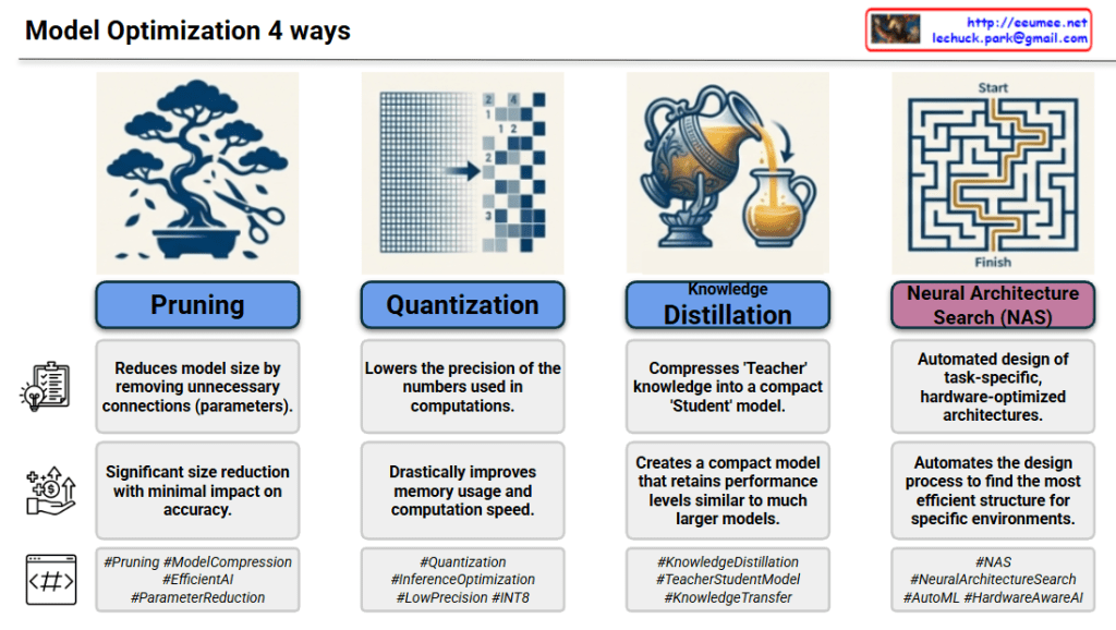
This diagram presents a learning and growth strategy for preparing for the AI era.
Core循環 Structure (Up Loop)
1. Make your base solid
The starting point of everything
Building strong fundamentals
2. Two developmental paths
Generalize from experience: Extract patterns and principles from your own experiences
Expand your generalizations: Extend existing understanding to broader domains
3. N × (Try & Fail)
Learning through iterative experimentation and failure
This process is the key to actual growth
4. The AI era
Ultimate goal: Adapt to and succeed in the AI era
5. Up Loop
Return to basics and repeat at a higher level
Continuous improvement and growth cycle
Supporting Principles (Bottom Section)
“Create your own definitions!! It’s okay to be a little wrong”
Create your own definitions
Being slightly wrong is acceptable (escape perfectionism)
“Think deeply and imagine boldly”
Think deeply and imagine courageously
“Build your network, Network with others”
The importance of building networks
These three elements combine → Strategy for AI Era
Key Message
This strategy emphasizes learning through continuous trial and error rather than perfection, self-directed learning, and networking. It aims to develop the competencies needed for the AI era through iterative improvement.
Summary
This framework advocates for a continuous learning cycle: build solid foundations, generalize and expand your knowledge, then embrace multiple failures as learning opportunities. The strategy rejects perfectionism in favor of bold experimentation, deep thinking, and collaborative networking. Success in the AI era comes from iterative improvement through this “up loop” rather than seeking perfect answers from the start.
How it works: Data flows sequentially like waves, with each GPU processing its assigned stage before passing to the next GPU.
Tensor Parallelism
Core Concept:
Matrix pool is prepared and split in advance
All GPUs simultaneously process different parts of the same data
Characteristics:
Axis: Width-wise – splits inside layers
Pattern: Width-wise sharding – splits matrix/attention across GPUs
Communication: Occurs at every Transformer layer (forward/backward)
Cost: High communication overhead, requires strong NVLink/NVSwitch
How it works: Large matrices are divided into chunks, with each GPU processing simultaneously while continuously communicating via NVLink/NVSwitch.
Key Differences
Aspect
Pipeline
Tensor
Split Method
Layer-wise (vertical)
Within-layer (horizontal)
GPU Role
Different tasks
Parts of same task
Communication
Low (stage boundaries)
High (every layer)
Hardware Needs
Standard
High-speed interconnect required
Summary
Pipeline Parallelism splits models vertically by layers with sequential processing and low communication cost, while Tensor Parallelism splits horizontally within layers for parallel processing but requires high-speed interconnects. These two techniques are often combined in training large-scale AI models to maximize efficiency.
This image illustrates a comprehensive Modular Data Center architecture designed specifically for modern AI/ML workloads, showcasing integrated systems and their key capabilities.
Core Components
1. Management Layer
Integrated Visibility: DCIM & Digital Twin for real-time monitoring
Autonomous Operations: AI-Driven Analytics (AIOps) for predictive maintenance
Physical Security: Biometric Access Control for enhanced protection
2. Computing Infrastructure
High Density AI Accelerators: GPU/NPU optimized for AI workloads
Scalability: OCP (Open Compute Project) Racks for standardized deployment
Standardization: High-Speed Interconnects (InfiniBand) for low-latency communication
3. Power Systems
Power Continuity: Modular UPS with Li-ion Battery for reliable uptime
Distribution Efficiency: Smart Busway/Busduct for optimized power delivery
Space Optimization: High-Voltage DC (HVDC) for reduced footprint
4. Cooling Solutions
Hot Spot Elimination: In-Row/Rear Door Cooling for targeted heat removal
PUE Optimization: Liquid/Immersion Cooling for maximum efficiency
High Heat Flux Handling: Containment Systems (Hot/Cold Aisle) for AI density
5. Safety & Environmental
Early Detection: VESDA (Very Early Smoke Detection Apparatus)
Environmental Monitoring: Leak Detection System (LDS)
Why Modular DC is Critical for AI Data Centers
Speed & Agility
Traditional data centers take 18-24 months to build, but AI demands are exploding NOW. Modular DCs deploy in 3-6 months, allowing organizations to capture market opportunities and respond to rapidly evolving AI compute requirements without lengthy construction cycles.
AI-Specific Thermal Challenges
AI workloads generate 3-5x more heat per rack (30-100kW) compared to traditional servers (5-10kW). Modular designs integrate advanced liquid cooling and containment systems from day one, purpose-built to handle GPU/NPU thermal density that would overwhelm conventional infrastructure.
Elastic Scalability
AI projects often start experimental but can scale exponentially. The “pay-as-you-grow” model lets organizations deploy one block initially, then add capacity incrementally as models grow—avoiding massive upfront capital while maintaining consistent architecture and avoiding stranded capacity.
Edge AI Deployment
AI inference increasingly happens at the edge for latency-sensitive applications (autonomous vehicles, smart manufacturing). Modular DCs’ compact, self-contained design enables AI deployment anywhere—from remote locations to urban centers—with full data center capabilities in a standardized package.
Operational Efficiency
AI workloads demand maximum PUE efficiency to manage operational costs. Modular DCs achieve PUE of 1.1-1.3 through integrated cooling optimization, HVDC power distribution, and AI-driven management—versus 1.5-2.0 in traditional facilities—critical when GPU clusters consume megawatts.
Key Advantages
📦 “All pack to one Block” – Complete infrastructure in pre-integrated modules 🧩 “Scale out with more blocks” – Linear, predictable expansion without redesign
⏱️ Time-to-Market: 4-6x faster deployment vs traditional builds
💰 Pay-as-you-Grow: CapEx aligned with revenue/demand curves
🌍 Anywhere & Edge: Containerized deployment for any location
Summary
Modular Data Centers are essential for AI infrastructure because they deliver pre-integrated, high-density compute, power, and cooling blocks that deploy 4-6x faster than traditional builds, enabling organizations to rapidly scale GPU clusters from prototype to production while maintaining optimal PUE efficiency and avoiding massive upfront capital investment in uncertain AI workload trajectories.
The modular approach specifically addresses AI’s unique challenges: extreme thermal density (30-100kW/rack), explosive demand growth, edge deployment requirements, and the need for liquid cooling integration—all packaged in standardized blocks that can be deployed anywhere in months rather than years.
This architecture transforms data center infrastructure from a multi-year construction project into an agile, scalable platform that matches the speed of AI innovation, allowing organizations to compete in the AI economy without betting the company on fixed infrastructure that may be obsolete before completion.
Parallelism Comparison: Data Parallelism vs Expert Parallelism
This image compares two major parallelization strategies used for training large language models (LLMs).
Left: Data Parallelism
Structure:
Data is divided into multiple batches from the database
Same complete model is replicated on each GPU
Each GPU independently processes different data batches
Results are aggregated to generate final output
Characteristics:
Scaling axis: Number of batches/samples
Pattern: Full model copy on each GPU, dense training
Communication: Gradient All-Reduce synchronization once per step
Advantages: Simple and intuitive implementation
Disadvantages: Model size must fit in single GPU memory
Right: Expert Parallelism
Structure:
Data is divided by layers
Tokens are distributed to appropriate experts through All-to-All network and router
Different expert models (A, B, C) are placed on each GPU
Parallel processing at block/thread level in GPU pool
Characteristics:
Scaling axis: Number of experts
Pattern: Sparse structure – only few experts activated per token
Goal: Maintain large capacity while limiting FLOPs per token
Communication: All-to-All token routing
Advantages: Can scale model capacity significantly (MoE – Mixture of Experts architecture)
Disadvantages: High communication overhead and complex load balancing
Key Differences
Aspect
Data Parallelism
Expert Parallelism
Model Division
Full model replication
Model divided into experts
Data Division
Batch-wise
Layer/token-wise
Communication Pattern
Gradient All-Reduce
Token All-to-All
Scalability
Proportional to data size
Proportional to expert count
Efficiency
Dense computation
Sparse computation (conditional activation)
These two approaches are often used together in practice, enabling ultra-large-scale model training through hybrid parallelization strategies.
Summary
Data Parallelism replicates the entire model across GPUs and divides the training data, synchronizing gradients after each step – simple but memory-limited. Expert Parallelism divides the model into specialized experts and routes tokens dynamically, enabling massive scale through sparse activation. Modern systems combine both strategies to train trillion-parameter models efficiently.
This image outlines the key technologies and performance efficiency of the DeepSeek-v3 model, which utilizes the Mixture-of-Experts (MoE) architecture. It is divided into the architecture diagram/cost table on the left and four key technical features on the right.
1. DeepSeekMoE Architecture (Left Diagram)
The diagram illustrates how the model processes data:
Separation of Experts: Unlike traditional MoEs, it distinguishes between Shared Experts (Green) and Routed Experts (Blue).
Shared Experts: Always active to handle common knowledge.
Routed Experts: Selectively activated by the Router to handle specific, specialized features.
Workflow: When an input (ut) arrives, the Router selects the top-$K$ experts (Top-Kr). The system processes the input through both shared and selected routed experts in parallel and combines the results.
2. Four Key Technical Features (Right Panel)
This section explains how DeepSeek-v3 overcomes the limitations of existing MoE models:
Load Balancing without Auxiliary Loss:
Problem: Standard MoEs often use “auxiliary loss” to balance expert usage, which can degrade performance.
Solution: It uses learnable bias terms in the router to ensure balance. This bias only affects “dispatching” (where data goes) and not the actual “weights” (calculation values), preserving model quality.
Shared Expert Design:
Concept: Keeping one or a few experts always active for general tasks allows the routed experts to focus purely on complex, specialized tasks.
Benefit: Reduces redundancy and improves the capacity utilization of experts.
Hardware-Aware Dual-Pipe Parallelism:
Efficiency: It fully overlaps All-to-All communication with computation, minimizing idle time.
Optimization: “Node-local expert routing” is used to minimize slow data transfers between different nodes.
FP8 Mixed-Precision Training:
Speed & Cost: Utilizes the tensor cores of modern GPUs (Hopper/Blackwell) for full FP8 (8-bit floating point) training. This drastically lowers both training and inference costs.
3. Cost Efficiency Comparison (Table 2)
The comparison highlights the massive efficiency gain over dense models:
DeepSeek-V3 MoE (671B parameters): Despite having the largest parameter count, its training cost is extremely low at 250 GFLOPS/Token.
LLaMa-405B Dense (405B parameters): Although smaller in size, it requires ~10x higher cost (2448 GFLOPS/Token) compared to DeepSeek-v3.
Conclusion: DeepSeek-v3 achieves “high performance at low cost” by massively scaling the model size (671B) while keeping the actual computation equivalent to a much smaller model.
Summary
Hybrid Structure: DeepSeek-v3 separates “Shared Experts” for general knowledge and “Routed Experts” for specialized tasks to maximize efficiency.
Optimized Training: It achieves high speed and balance using “Load Balancing without Auxiliary Loss” and “FP8 Mixed-Precision Training.”
Extreme Efficiency: Despite a massive 671B parameter size, it offers roughly 10x lower training costs per token compared to similar dense models (like LLaMa-405B).