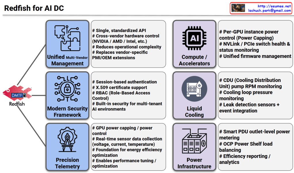
Basic LLM Workflow

Basic LLM Workflow Interpretation

This diagram illustrates how data flows through various hardware components during the inference process of a Large Language Model (LLM).

Step-by-Step Breakdown

① Initialization Phase (Warm weights)

  • Model weights are loaded from SSD → DRAM → HBM (High Bandwidth Memory)
  • Weights are distributed and shared across multiple GPUs

② Input Processing (CPU tokenizes/batches)

  • CPU tokenizes input text and processes batches
  • Data is transferred through DRAM buffer to GPU

③ GPU Inference Execution

  • GPU performs Attention and FFN (Feed-Forward Network) computations from HBM
  • KV cache (Key-Value cache) is stored in HBM
  • If HBM is tight, KV cache can be offloaded to DRAM or SSD

④ Distributed Communication (NvLink/Infiniband)

  • Intra-node: High-speed communication between GPUs via NvLink (with NVSwitch if available)
  • Inter-node: Parallel communication through InfiniBand or NCCL

⑤ Post-processing (CPU decoding/post)

  • CPU decodes generated tokens and performs post-processing
  • Logs and caches are saved to SSD

Key Characteristics

This architecture leverages a memory hierarchy to efficiently execute large-scale models:

  • SSD: Long-term storage (slowest, largest capacity)
  • DRAM: Intermediate buffer
  • HBM: GPU-dedicated high-speed memory (fastest, limited capacity)

When model size exceeds GPU memory, strategies include distributing across multiple GPUs or offloading data to higher-level memory tiers.


Summary

This diagram shows how LLMs process data through a memory hierarchy (SSD→DRAM→HBM) across CPU and GPU components. The workflow involves loading model weights, tokenizing inputs on CPU, running inference on GPU with HBM, and using distributed communication (NvLink/InfiniBand) for multi-GPU setups. Memory management strategies like KV cache offloading enable efficient execution of large models that exceed single GPU capacity.

#LLM #DeepLearning #GPUComputing #MachineLearning #AIInfrastructure #NeuralNetworks #DistributedComputing #HPC #ModelOptimization #AIArchitecture #NvLink #Transformer #MLOps #AIEngineering #ComputerArchitecture

With Claude

The Perfect Paradox

The Perfect Paradox – Analysis

This diagram illustrates “The Perfect Paradox”, explaining the relationship between effort and results. Here are the key concepts:

Graph Analysis

Axes:

  • X-axis: Effort
  • Y-axis: Result

Pattern:

  • Initially, results increase proportionally with effort
  • After the Inflection Point (green circle), dramatically increased effort yields minimal or even diminishing returns
  • “Perfect” exists in an unreachable zone

Core Message

“Good Enough (Satisfying)”

  • Located near the inflection point
  • Represents the optimal effort-to-result ratio

The Central Paradox:

“Before ‘perfect’ lies ‘infinite’.”

This means achieving perfection requires infinite effort.

AI Connection

The bottom arrow shows the evolution of approaches:

  • Rule-based ApproachData-Driven Approach

Key Insight:

“While data-driven AI is now far beyond ‘good enough’, it remains imperfect.”

This suggests that modern AI achieves high performance, but pursuing practical utility is more rational than chasing perfection.


Summary

The Perfect Paradox shows that after a certain inflection point, exponentially more effort produces minimal improvement, making “perfect” practically unreachable. The optimal strategy is achieving “good enough” – the sweet spot where effort and results are balanced. Modern data-driven AI has surpassed “good enough” but remains imperfect, demonstrating that practical excellence trumps impossible perfection.

#PerfectParadox #DiminishingReturns #GoodEnough #EffortVsResults #PracticalExcellence #AILimitations #DataDrivenAI #InflectionPoint #OptimizationStrategy #PerfectionismVsPragmatism #ProductivityInsights #SmartEffort #AIPhilosophy #EfficiencyMatters #RealisticGoals

AI-driven operational intelligence loop

AI-Driven Operational Intelligence Loop


1️⃣ High-Resolution & Accurate Data


Collect precise, high-frequency sensor data across all systems to ensure reliability and synchronization.

2️⃣ Change Detection & Connectivity


Continuously monitor data variations and correlations to identify anomalies and causal relationships in real time.

3️⃣ Analytics & Classification


Analyze detected changes, classify events by impact and severity, and generate actionable insights for optimization.

4️⃣ Response Framework


Define and execute automated or semi-automated response strategies based on analysis and classification results.

5️⃣ AI Application & Continuous Learning


Use AI to automate steps 2–4, enhance prediction accuracy, and continuously improve operations through feedback and model retraining.

Loop Concept
1 Data → 2 Detection → 3 Analysis → 4 Response → 5 AI → (Feedback & Optimization)
Goal:
Build a self-optimizing operational ecosystem that integrates data, AI, and automation for smarter, more reliable digital operations.

Operations by Metrics

1. Big Data Collection & 2. Quality Verification

  • Big Data Collection: Represented by the binary data (top-left) and the “All Data (Metrics)” block (bottom-left).
  • Data Quality Verification: The collected data then passes through the checklist icon (top flow) and the “Verification (with Resolution)” step (bottom flow). This aligns with the quality verification step, including ‘resolution/performance’.

3. Change Data Capture (CDC)

  • Verified data moves to the “Change Only” stage (central pink box).
  • If there are “No Changes,” it results in “No Actions,” illustrating the CDC (Change Data Capture) concept of processing only altered data.
  • The magnifying glass icon in the top flow also visualizes this ‘change detection’ role.

4. State/Numeric Processing & 5. Analysis, Severity Definition

  • State/Numeric Processing: Once changes are detected (after the magnifying glass), the data is split into two types:
    • State Changes (ON/OFF icon): Represents changes in ‘state values’.
    • Numeric Changes (graph icon): Represents changes in ‘numeric values’.
  • Statistical Analysis & Severity Definition:
    • These changes are fed into the “Analysis” step.
    • This stage calculates the “Count of Changes” (statistics on the number of changes) and “Numeric change Diff” (amount of numeric change).
    • The analysis result leads to “Severity Tagging” to define the ‘Severity’ level (e.g., “Critical? Major? Minor?”).

6. Notification & 7. Analysis (Retrieve)

  • Notification: Once the severity is defined, the “Notification” step (bell/email icon) is triggered to alert personnel.
  • Analysis (Retrieve):
    • The notified user then performs the “Retrieve” action.
    • This final step involves querying both the changed data (CDD results) and the original data (source, indicated by the URL in the top-right) to analyze the cause.

Summary

This workflow begins with collecting and verifying all data, then uses CDC to isolate only the changes. These changes (state or numeric) are analyzed for count and difference to assign a severity level. The process concludes with notification and a retrieval step for root cause analysis.

#DataProcessing #DataMonitoring #ChangeDataCapture #CDC #DataAnalysis #SystemMonitoring #Alerting #ITOperations #SeverityAnalysis

With Gemini

AI Operation : All Connected

AI Operation: All Connected – Image Analysis

This diagram explains the operational paradigm shift in AI Data Centers (AI DC).

Top Section: New Challenges

AI DC Characteristics:

  • Paradigm shift: Fundamental change in operations for the AI era
  • High Cost: Massive investment required for GPUs, infrastructure, etc.
  • High Risk: Greater impact during outages and increased complexity

Five Core Components of AI DC (left→right):

  1. Software: AI models, application development
  2. Computing: GPUs, servers, and computational resources
  3. Network: Data transmission and communication infrastructure
  4. Power: High-density power supply and management (highlighted in orange)
  5. Cooling: Heat management and cooling systems

→ These five elements are interconnected through the “All Connected Metric”

Bottom Section: Integrated Operations Solution

Core Concept:

📦 Tightly Fused Rubik’s Cube

  • The five core components (Software, Computing, Network, Power, Cooling) are intricately intertwined like a Rubik’s cube
  • Changes or issues in one element affect all other elements due to tight coupling

🎯 All Connected Data-Driven Operations

  • Data-driven integrated operations: Collecting and analyzing data from all connected elements
  • “For AI, With AI”: Operating the data center itself using AI technology for AI workloads

Continuous Stability & Optimization

  • Ensuring continuous stability
  • Real-time monitoring and optimization

Key Message

AI data centers have five core components—Software, Computing, Network, Power, and Cooling—that are tightly fused together. To effectively manage this complex system, a data-centric approach that integrates and analyzes data from all components is essential, enabling continuous stability and optimization.


Summary

AI data centers are characterized by tightly coupled components (software, computing, network, power, cooling) that create high complexity, cost, and risk. This interconnected system requires data-driven operations that leverage AI to monitor and optimize all elements simultaneously. The goal is achieving continuous stability and optimization through integrated, real-time management of all connected metrics.

#AIDataCenter #DataDrivenOps #AIInfrastructure #DataCenterOptimization #TightlyFused #AIOperations #HybridInfrastructure #IntelligentOps #AIforAI #DataCenterManagement #MLOps #AIOps #PowerManagement #CoolingOptimization #NetworkInfrastructure

Multi-Token Prediction (MTP) – Increasing Inference Speed

This image explains the Multi-Token Prediction (MTP) architecture that improves inference speed.

Overall Structure

Left: Main Model

  • Starts with an Embedding Layer that converts input tokens to vectors
  • Deep neural network composed of L Transformer Blocks
  • RMSNorm stabilizes the range of Transformer input/output values
  • Finally, the Output Head (BF16 precision) calculates the probability distribution for the next token

Right: MTP Module 1 (Speculative Decoding Module) + More MTP Modules

  • Maximizes efficiency by reusing the Main Model’s outputs
  • Two RMSNorms normalize the intermediate outputs from the Main Model
  • Performs lightweight operations using a single Transformer Block with FP8 Mixed Precision
  • Generates specialized vectors for future token prediction through Linear Projection and concatenation
  • Produces candidate tokens with BF16 precision

Key Features

  1. Two-stage processing: The Main Model accurately predicts the next token, while the MTP Module generates additional candidate tokens in advance
  2. Efficiency:
    • Shares the Embedding Layer with the Main Model to avoid recalculation
    • Reduces computational load with FP8 Mixed Precision
    • Uses only a single Transformer Block
  3. Stability: RMSNorm ensures stable processing of outputs that haven’t passed through the Main Model’s deep layers

Summary

MTP architecture accelerates inference by using a lightweight module alongside the main model to speculatively generate multiple future tokens in parallel. It achieves efficiency through shared embeddings, mixed precision operations, and a single transformer block while maintaining stability through normalization layers. This approach significantly reduces latency in large language model generation.

#MultiTokenPrediction #MTP #SpeculativeDecoding #LLM #TransformerOptimization #InferenceAcceleration #MixedPrecision #AIEfficiency #NeuralNetworks #DeepLearning

With Claude