FP8 Mixed-Precision Training Interpretation
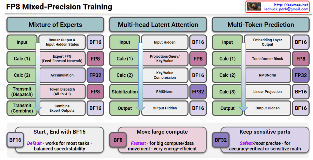
This image is a technical diagram showing FP8 (8-bit Floating Point) Mixed-Precision Training methodology.
Three Main Architectures
1. Mixture of Experts (MoE)
- Input: Starts with BF16 precision
- Calc (1): Router output & input hidden states → BF16
- Calc (2): Expert FFN (Feed-Forward Network) → FP8 computation
- Calc (3): Accumulation → FP32
- Transmit (Dispatch): Token dispatch (All-to-All) → FP8
- Transmit (Combine): Combine expert outputs → BF16
- Output: BF16
2. Multi-head Latent Attention
- Input: BF16
- Calc (1): Input hidden states → BF16
- Calc (2): Projection/Query/Key/Value → FP8
- Calc (3): Key/Value compression → BF16
- Stabilization: RMSNorm → FP32
- Output: Output hidden states → BF16
3. Multi-Token Prediction
- Input: BF16
- Calc (1): Embedding layer output → BF16
- Calc (2): Transformer block → FP8
- Calc (3): RMSNorm → FP32
- Calc (4): Linear projection → BF16
- Output: Output hidden states → BF16
Precision Strategy (Bottom Boxes)
🟦 BF16 (Default)
- Works for most tasks
- Balanced speed/stability
🟪 BF8 (Fastest)
- For large compute/data movement
- Very energy-efficient
🟣 BF32 (Safest/Most Precise)
- For accuracy-critical or sensitive math operations
Summary
FP8 mixed-precision training strategically uses different numerical precisions across model operations: FP8 for compute-intensive operations (FFN, attention, transformers) to maximize speed and efficiency, FP32 for sensitive operations like accumulation and normalization to maintain numerical stability, and BF16 for input/output and communication to balance performance. This approach enables faster training with lower energy consumption while preserving model accuracy, making it ideal for training large-scale AI models efficiently.
#FP8Training #MixedPrecision #AIOptimization #DeepLearning #ModelEfficiency #NeuralNetworks #ComputeOptimization #MLPerformance #TransformerTraining #EfficientAI #LowPrecisionTraining #AIInfrastructure #MachineLearning #GPUOptimization #ModelTraining
With Claude