Corpus, Ontology and LLM

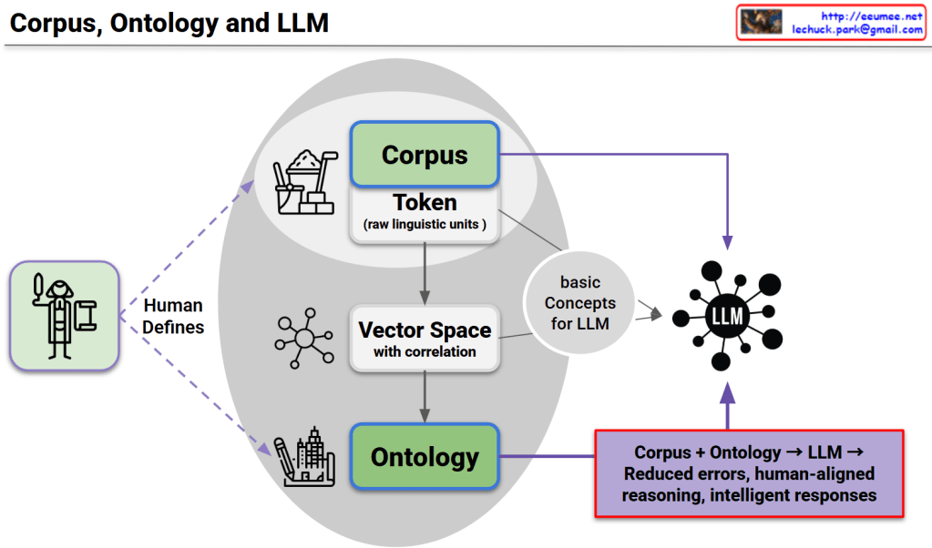
This diagram presents a unified framework consisting of three core structures, their interconnected relationships, and complementary utilization as the foundation for LLM advancement.

Three Core Structures

1. Corpus Structure

  • Token-based raw linguistic data
  • Provides statistical language patterns and usage frequency information

2. Ontology Structure

  • Systematically human-defined conceptual knowledge structure
  • Provides logical relationships and semantic hierarchies

3. LLM Structure

  • Neural network-based language processing model
  • Possesses pattern learning and generation capabilities

Interconnected Relationships and Interactions

  • Corpus → Vector Space: Numerical representation transformation of linguistic data
  • Ontology → Basic Concepts: Conceptual abstraction of structured knowledge
  • Vector Space ↔ Ontology: Mutual validation between statistical patterns and logical structures
  • Integrated Concepts → LLM: Multi-layered knowledge input

LLM Development Foundation through Complementary Relationships

Each structure compensates for the limitations of others:

  • Corpus’s statistical accuracy + Ontology’s logical consistency → Balanced knowledge foundation
  • Ontology’s explicit rules + LLM’s pattern learning → Flexible yet systematic reasoning
  • Corpus’s real-usage data + LLM’s generative capability → Natural and accurate language generation

Final Achievement

This triangular complementary structure overcomes the limitations of single approaches to achieve:

  • Error minimization
  • Human-centered reasoning capabilities
  • Intelligent and reliable response generation

This represents the core foundation for next-generation LLM development.

With Claude

go with : the best efficient

System Operations Strategy: Stabilize vs Optimize Analysis

Graph Components

Operational Performance Levels (Color-coded meanings):

  • Blue Line: Risk Zone – Abnormal operational state requiring urgent intervention
  • Green Line: Stable and efficient ideal operational range
  • Purple Line: Enhanced high-performance operational state
  • Dark Red Line: Fully optimized peak performance state
  • Gray Line: Conservative stable operation (high cost consumption)

Core Operating Philosophy

Phase 1: Stabilize

Objective: keep <Green> higher than <Blue>

  • Meaning: Build defense mechanisms to prevent system from falling below risk zone (blue)
  • Impact: Prevent failures, ensure service continuity
  • Approach: Proactive response through predictive-based prevention, prioritizing stability

Phase 2: Optimize

Objective: move <Green> to <Red>

  • Meaning: Gradual performance improvement on a stabilized foundation
  • Impact: Simultaneous improvement of cost efficiency and operational performance
  • Approach: Pursue optimization within limits that don’t compromise stability

Strategic Insights

1. Importance of Sequential Approach

  • The Stabilize → Optimize sequence is essential
  • Direct optimization without stabilization increases risk exposure

2. Cost Efficiency Paradox

  • Stable efficiency (green) is practically more valuable than full optimization (red)
  • Excessive optimization can result in diminishing returns on investment

3. Dynamic Equilibrium Maintenance

  • Green zone represents a dynamic benchmark continuously adjusted upward, not a fixed target
  • Balance point between stability and efficiency must be continuously recalibrated based on environmental changes

Practical Implications

This model visualizes the core principle of modern system operations: “Stability is the prerequisite for efficiency.” Rather than pursuing performance improvements alone, it presents strategic guidelines for achieving genuine operational efficiency through gradual and sustainable optimization built upon a solid foundation of stability.

The framework emphasizes that true operational excellence comes not from aggressive optimization, but from maintaining the optimal balance between risk mitigation and performance enhancement, ensuring long-term business value creation through sustainable operational practices.

With Claude

Memory Bound

This diagram illustrates the Memory Bound phenomenon in computer systems.

What is Memory Bound?

Memory bound refers to a situation where the overall processing speed of a computer is limited not by the computational power of the CPU, but by the rate at which data can be read from memory.

Main Causes:

  1. Large-scale Data Processing: Vast data volumes cause delays when loading data from storage devices (SSD/HDD) to DRAM
  2. Matrix Operations: Large matrices create delays in fetching data between cache, DRAM, and HBM (High Bandwidth Memory)
  3. Data Copying/Moving: Data transfer waiting times on the memory bus even within DRAM
  4. Cache Misses: When required data isn’t found in L1-L3 caches, causing slow main memory access to DRAM

Result

The Processing Elements (PEs) on the right have high computational capabilities, but the overall system performance is constrained by the slower speed of data retrieval from memory.

Summary:

Memory bound occurs when system performance is limited by memory access speed rather than computational power. This bottleneck commonly arises from large data transfers, cache misses, and memory bandwidth constraints. It represents a critical challenge in modern computing, particularly affecting GPU computing and AI/ML workloads where processing units often wait for data rather than performing calculations.

With Claude