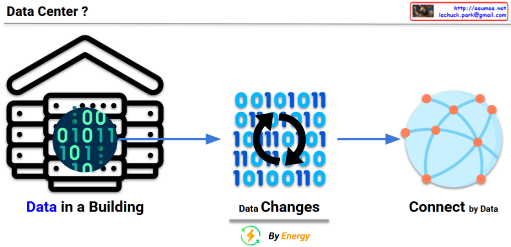
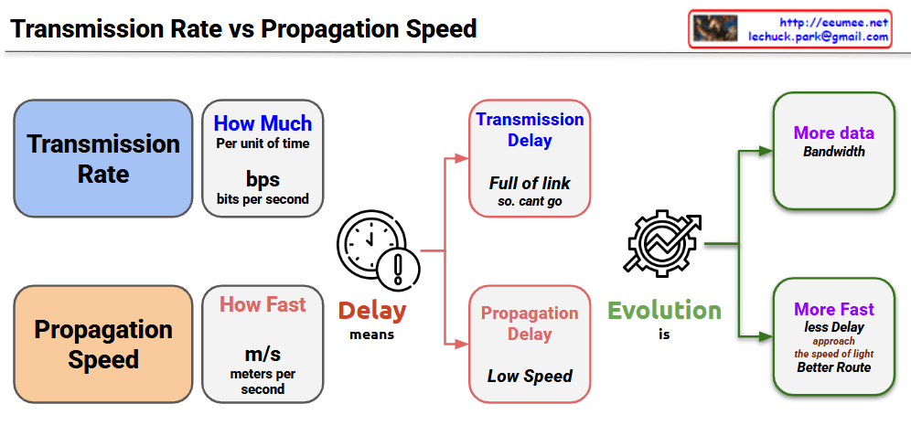
Transmission Rate vs Propagation Speed

Key Concepts

Transmission Rate

  • Amount of data processable per unit time (bps – bits per second)
  • “Processing speed” concept – how much data can be handled simultaneously
  • Low transmission rate causes Transmission Delay
  • “Link is full, cannot send data”

Propagation Speed

  • Speed of signal movement through physical media (m/s – meters per second)
  • “Travel speed” concept – how fast signals move
  • Slow propagation speed causes Propagation Delay
  • “Arrives late due to long distance”

Meaning of Delay

Two types of delays affect network performance through different principles. Transmission delay is packet size divided by transmission rate – the time to push data into the link. Propagation delay is distance divided by propagation speed – the time for signals to physically travel.

Two Directions of Technology Evolution

Bandwidth Expansion (More Data Bandwidth)

  • Improved data processing capability through transmission rate enhancement
  • Development of high-speed transmission technologies like optical fiber and 5G
  • No theoretical limits – continuous improvement possible

Path Optimization (More Fast, Less Delay)

  • Faster response times through propagation delay improvement
  • Physical distance reduction, edge computing, optimal routing
  • Fundamental physical limits exist: cannot exceed speed of light (c = 3×10⁸ m/s)
  • Actual media is slower due to refractive index (optical fiber: ~2×10⁸ m/s)

Network communication involves two distinct “speed” concepts: Transmission Rate (how much data can be processed per unit time in bps) and Propagation Speed (how fast signals physically travel in m/s). While transmission rate can be improved infinitely through technological advancement, propagation speed faces an absolute physical limit – the speed of light – creating fundamentally different approaches to network optimization. Understanding this distinction is crucial because transmission delays require bandwidth solutions, while propagation delays require path optimization within unchangeable physical constraints.

With Claude

Key Factors in DC

This image is a diagram showing the key components of a Data Center (DC).

The diagram visually represents the core elements that make up a data center:

  1. Building – Shown on the left with a building icon, representing the physical structure of the data center.
  2. Core infrastructure elements (in the central blue area):
    • Network – Data communication infrastructure
    • Computing – Servers and processing equipment
    • Power – Energy supply systems
    • Cooling – Temperature regulation systems
  3. The central orange circle represents server racks, which is connected to power supply units (transformers), cooling equipment, and network devices.
  4. Digital Service – Displayed on the right, representing the end services that all this infrastructure ultimately delivers.

This diagram illustrates how a data center flows from a physical building through core elements like network, computing, power, and cooling to ultimately provide digital services.

With Claude

Data Center

This image explains the fundamental concept and function of a data center:

  1. Left: “Data in a Building” – Illustrates a data center as a physical building that houses digital data (represented by binary code of 0s and 1s).
  2. Center: “Data Changes” – With the caption “By Energy,” showing how data is processed and transformed through the consumption of energy.
  3. Right: “Connect by Data” – Demonstrates how processed data from the data center connects to the outside world, particularly the internet, forming networks.

This diagram visualizes the essential definition of a data center – a physical building that stores data, consumes energy to process that data, and plays a crucial role in connecting this data to the external world through the internet.

With Claude

TCP Challenge ACK

This image explains the TCP Challenge ACK mechanism.

At the top, it shows a normal “TCP Connection Established” state. Below that, it illustrates two attack scenarios and the defense mechanism:

  1. First scenario: An attacker sends a SYN packet with SEQ(attack) value to an already connected session. The server responds with a TCP Challenge ACK.
  2. Second scenario: An attacker sends an RST packet with SEQ(attack) value. The server checks if the SEQ(attack) value is within the receive window size (RECV_WIN_SIZE):
    • If the value is inside the window (YES) – The session is reset.
    • If the value is outside the window (NO) – A TCP Challenge ACK is sent.

Additional information at the bottom includes:

  • The Challenge ACK is generated in the format seed ACK = SEQ(attack)+@
  • The net.ipv4.tcp_challenge_ack_limit setting indicates the limit number of TCP Challenge ACKs sent per second, which is used to block RST DDoS attacks.

Necessity and Effectiveness of TCP Challenge ACK:

TCP Challenge ACK is a critical mechanism for enhancing network security. Its necessity and effectiveness include:

  • Preventing Connection Hijacking: Detects and blocks attempts by attackers trying to hijack legitimate TCP connections.
  • Session Protection: Protects existing TCP sessions from RST/SYN packets with invalid sequence numbers.
  • Attack Validation: Verifies the authenticity of packets through Challenge ACKs, preventing connection termination by malicious packets.
  • DDoS Mitigation: Protects systems from RST flood attacks that maliciously terminate TCP connections.
  • Defense Against Blind Attacks: Increases the difficulty of blind attacks by requiring attackers to correctly guess the exact sequence numbers for successful attacks.

With Claude

Data Center NOW

This image shows a data center architecture diagram titled “Data Center Now” at the top. It illustrates the key components and flow of a modern data center infrastructure.

The diagram depicts:

  1. On the left side: An “Explosion of data” icon with data storage symbols, pointing to computing components with the note “More Computing is required”
  2. In the center: Server racks connected to various systems with colored lines indicating different connections (red, blue, green)
  3. On the right side: Several technology components illustrated with circular icons and labels:
    • “Software Defined” with a computer/gear icon
    • “AI & GPU” with neural network and GPU icons and note “Big power is required”
    • “Renewable Energy & Grid Power” with solar panel and wind turbine icons
    • “Optimized Cooling /w Using Water” with cooling system icon
    • “Enhanced Op System & AI Agent” with a robotic/AI system icon

The diagram shows how data flows through processing units and connects to different infrastructure elements, emphasizing modern data center requirements like increased computing power, AI capabilities, power management, and cooling solutions.

With Claude

NAPI

This image shows a diagram of the Network New API (NAPI) introduced in Linux kernel 2.6. The diagram outlines the key components and concepts of NAPI with the following elements:

The diagram is organized into several sections:

  1. NAPI – The main concept is highlighted in a purple box
  2. Hybrid Mode – In a red box, showing the combination of interrupt and polling mechanisms
  3. Interrupt – In a green box, described as “to detect packet arrival”
  4. Polling – In a blue box, described as “to process packets in batches”

The Hybrid Mode section details four key features:

  1. <Interrupt> First – For initial packet detection
  2. <Polling> Mode – For interrupt mitigation
  3. Fast Packet Processing – For multi-packet processing in one time
  4. Load Balancing – For parallel processing with multiple cores

On the left, there’s a yellow box explaining “Optimizing interrupts during FAST Processing”

The bottom right contains additional information about prioritizing and efficiently allocating resources to process critical tasks quickly, accompanied by warning/hand and target icons.

The diagram illustrates how NAPI combines interrupt-driven and polling mechanisms to efficiently handle network packet processing in Linux.

With Claude

Traffic Control

This image shows a network traffic control system architecture. Here’s a detailed breakdown:

  1. At the top, several key technologies are listed:
  • P4 (Programming Protocol-Independent Packet Processors)
  • eBPF (Extended Berkeley Packet Filter)
  • SDN (Software-Defined Networking)
  • DPI (Deep Packet Inspection)
  • NetFlow/sFlow/IPFIX
  • AI/ML-Based Traffic Analysis
  1. The system architecture is divided into main sections:
  • Traffic flow through IN PORT and OUT PORT
  • Routing based on Destination IP address
  • Inside TCP/IP and over TCP/IP sections
  • Security-Related Conditions
  • Analysis
  • AI/ML-Based Traffic Analysis
  1. Detailed features:
  • Inside TCP/IP: TCP/UDP Flags, IP TOS (Type of Service), VLAN Tags, MPLS Labels
  • Over TCP/IP: HTTP/HTTPS Headers, DNS Queries, TLS/SSL Information, API Endpoints
  • Security-Related: Malicious Traffic Patterns, Encryption Status
  • Analysis: Time-Based Conditions, Traffic Patterns, Network State Information
  1. The AI/ML-Based Traffic Analysis section shows:
  • AI/ML technologies learn traffic patterns
  • Detection of anomalies
  • Traffic control based on specific conditions

This diagram represents a comprehensive approach to modern network monitoring and control, integrating traditional networking technologies with advanced AI/ML capabilities. The system shows a complete flow from packet ingress to analysis, incorporating various layers of inspection and control mechanisms.

with Claude