From DALL-E with some prompting The flowchart illustrates a four-step network anomaly detection process:
Data Collection: Gather various types of network data.
Protocol Usage: Employ SNMP, SFLOW/NETFLOW, and other methods to extract the data.
Analysis: Analyze Ethernet and TCP/IP header data for irregularities.
Control: Implement countermeasures like blocking traffic or controlling specific IP addresses.
The expected benefits of this process include enhanced network security through early detection of anomalies, the ability to prevent potential breaches by blocking suspicious traffic, and improved network management via real-time analysis and control.
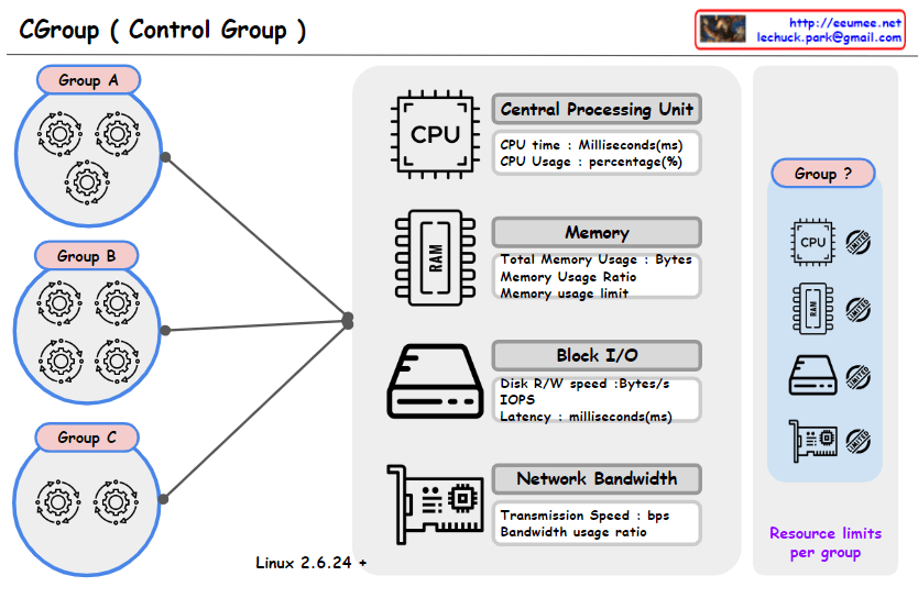
This image represents a concept diagram for ‘Control Groups’ (Cgroups) used in the Linux operating system. Cgroups provide the capability to manage and limit system resource usage for groups of processes. Each control group can have limits set for various resources such as CPU, memory, block I/O, and network bandwidth.
Groups A, B, C: Each circle represents a separate control group, and the gear icons within each group symbolize the processes assigned to that group.
The central graphical elements represent various system resources:
CPU: Represents CPU time and usage (milliseconds, percentage). Memory (RAM): Shows total memory usage, memory usage ratio, and memory usage limit. Block I/O: Illustrates disk read/write speed, number of input/output operations per second (IOPS), and latency. Network Bandwidth: Displays transmission speed and bandwidth usage ratio. In the upper right, there’s a section with the text “Resource limits per group” alongside icons for each resource and a question-marked group. This likely illustrates the resource limitations that can be set for each control group.
At the bottom, “Linux 2.6.24 +” indicates that the Cgroups feature is available from Linux kernel version 2.6.24 onwards.
Overall, the image seems to have been created to explain the concept of Cgroups and how resources can be managed for different groups within a system.
+ 224.0.0.6 (All Designated Routers) : Designated Router (DR) and Backup Designated Router (BDR). It is utilized to optimize communication between the DR and BDR, and regular OSPF routers do not receive messages from this address.
From DALL-E with Some prompting The image is a visual representation of the operation of the OSPF (Open Shortest Path First) protocol. Here is the interpretation of each step depicted in the image:
get LS (Link State): OSPF routers collect cost values from all physically connected routers. This step involves determining the adjacency relationships between routers and the state of each link.
LSA (Link State Advertisement): Each router creates an LSA that contains its link-state information and disseminates it to other routers within the network. During this process, the multicast address 224.0.0.5 is used to broadcast the information to all OSPF routers.
LSDB (Link State Database): The information from the received LSAs is compiled into the LSDB of every OSPF router. This database should be identical across all routers within the Autonomous System (AS) and contains the complete topology information of the network.
Shortest Path Tree Calculation: Using the LSDB, each router calculates the shortest path tree from itself to all other destinations employing the Dijkstra algorithm. This calculation aids each router in determining the optimal routing paths.
Routing Table Update: The shortest path information calculated is then used to update the routing table of each router. This enables routers to forward packets using the optimal routes.
At the bottom, there’s a section titled Dynamic Updates, indicating that when there are changes in the network topology, new LSAs are generated and propagated through the network. This ensures that all routers’ LSDBs are updated and, as a result, the routing tables are also updated to reflect the new optimal routes.
In the top-right corner, it states “224.0.0.5 Broadcast IP for all OSPF router”, which indicates the multicast address used by all OSPF routers to receive LSA broadcasts.
This diagram provides a visual explanation of the core routing processes of OSPF, highlighting the mechanisms that enable efficient routing within the network and facilitate rapid convergence.
Linear Regression: Yields a continuous output. Relates independent variable X with dependent variable Y through a linear relationship. Uses Mean Squared Error (MSE) as a performance metric. Can be extended to Multi-linear Regression for multiple independent variables.
Linear & Logistic Regression
The process begins with data input, as indicated by “from Data.”
Machine learning algorithms then process this data.
The outcome of this process branches into two types of regression, as indicated by “get Functions.”
Logistics Regression: Used for classification tasks, distinguishing between two or more categories. Outputs a probability percentage (between 0 or 1) indicating the likelihood of belonging to a particular class. Performance is evaluated using Log Loss or Binary Cross-Entropy metrics. Can be generalized to Softmax/Multinomial Logistic Regression for multi-class classification problems.
The image also graphically differentiates the two types of regression. Linear Regression is represented with a scatter plot and a trend line indicating the predictive linear equation. Logistic Regression is shown with a sigmoid function curve that distinguishes between two classes, highlighting the model’s ability to classify data points based on the probability threshold.
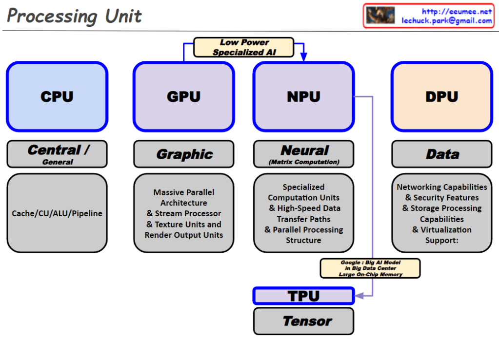
NPU and TPU are differentiated by their low power, specialized AI purpose.
TPU is developed by Google for large AI models in big data centers and features large on-chip memory.
The diagram emphasizes the specialized nature of NPU and TPU for AI tasks, highlighting their low power consumption and specialized computation capabilities, particularly for neural and tensor computations. It also contrasts these with the more general-purpose capabilities of CPUs and the graphic processing orientation of GPUs. DPU is presented as specialized for handling data-centric tasks involving networking, security, and storage in virtualized environments.
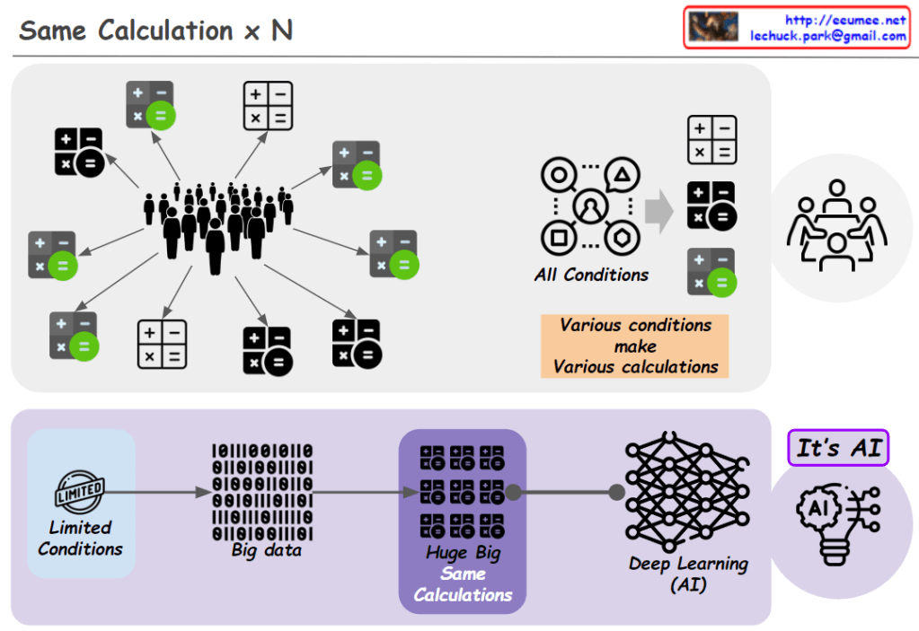
From DALL-E with some prompting The image illustrates the evolution from traditional computational methods to AI, emphasizing how initially, human computations were limited by the inability to quantify all conditions, leading to varied outcomes. Through discussion, the most rational results were derived. In contrast, AI operates on big data (which is inherently limited since it is pre-defined data) and implements intelligence through an enormous number of identical calculations, showcasing the capabilities of AI to handle vast and complex datasets and perform sophisticated analyses leading to innovative solutions.