DNS Caching SEQ

From Claude with some prompting
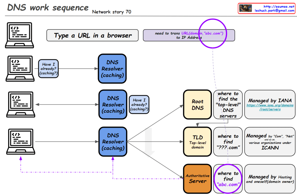
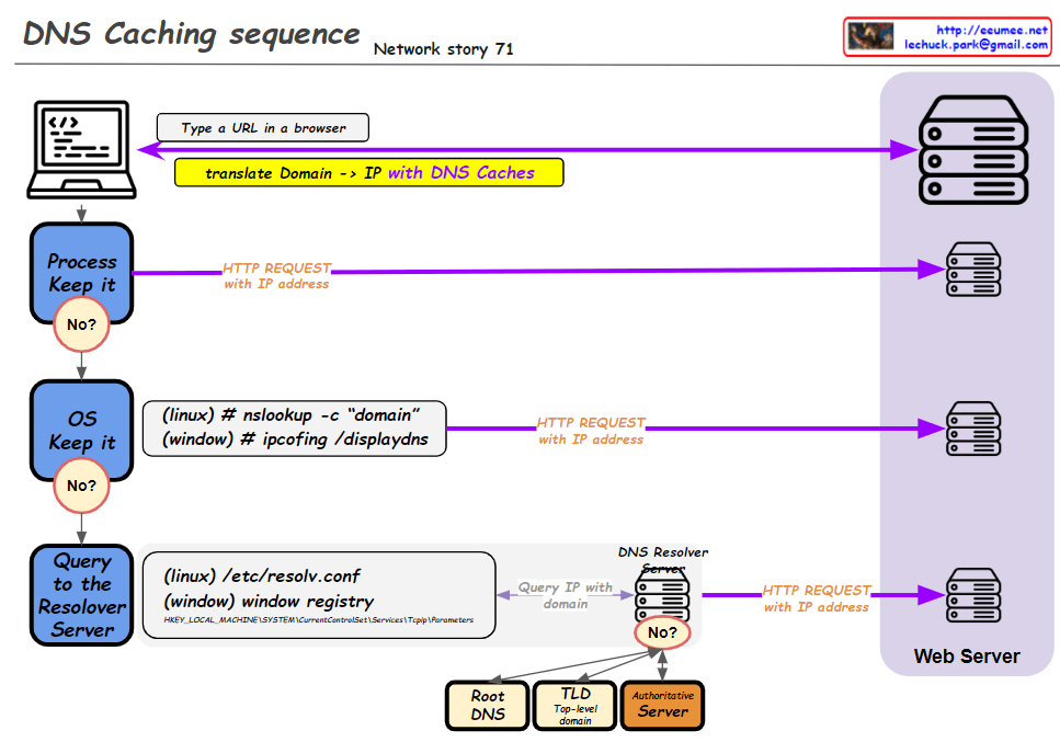
This improved diagram illustrates the DNS caching sequence more comprehensively. Here’s a breakdown of the process:

  1. A user types a URL in a browser.
  2. The system attempts to translate the domain to an IP address using DNS caches.
  3. Process Keep it: Checks the process-level DNS cache. If the information isn’t found here (“No”), it moves to the next step.
  4. OS Keep it: Checks the operating system-level DNS cache. For Linux, it uses the “nslookup -c domain” command, while for Windows, it uses “ipconfig /displaydns”. If the information isn’t found here (“No”), it proceeds to the next step.
  5. Query to the Resolver Server: The system queries the DNS resolver server. The resolver’s information is found in “/etc/resolv.conf” for Linux or the Windows Registry for Windows systems.
  6. If the resolver doesn’t have the information cached (“No”), it initiates a recursive query through the DNS hierarchy:
    • Root DNS
    • TLD (Top-Level Domain) server
    • Authoritative server
  7. Once the IP address is obtained, an HTTP request is sent to the web server.

This diagram effectively shows the hierarchical nature of DNS resolution and the fallback mechanisms at each level. It demonstrates how the system progressively moves from local caches to broader, more authoritative sources when resolving domain names to IP addresses. The addition of the DNS hierarchy (Root, TLD, Authoritative) provides a more complete picture of the entire resolution process when local caches and the initial resolver query don’t yield results.

DNS work sequence

From Claude with some prompting
This image illustrates the DNS (Domain Name System) work sequence. Here’s a breakdown:

  1. It starts with typing a URL in a browser. For example, entering “abc.com” requires translation to an IP address.
  2. The DNS resolution process begins, involving multiple levels of DNS resolvers with caching capabilities.
  3. At each level, there’s a “Have I already? (caching?)” check. If the information is cached, it’s used immediately.
  4. If not found, it proceeds to the next level:
    • Root DNS: Provides information on top-level DNS servers (Managed by IANA)
    • TLD (Top-Level Domain): Gives information on domains like “.com” (Managed by various organizations under ICANN)
    • Authoritative Server: Provides actual domain information (e.g., abc.com, managed by hosting providers or domain owners)
  5. Through these stages, the system finds the necessary information to ultimately obtain the IP address of the entered domain.

This diagram effectively demonstrates the hierarchical structure of DNS lookup process and the caching mechanism at each stage.

DNS Why?

From Claude with some prompting
This image is a network diagram explaining the function and importance of DNS (Domain Name System). The main points are:

  1. WWW service works with DNS on TCP/IP.
  2. DNS is responsible for mapping domains to IP addresses.
  3. All network devices on the Internet can only route to IP addresses.
  4. It’s difficult to include actual service characteristics in IP addresses (only by number).
  5. Domain addresses are easy to use and must be mapped to IP addresses.
  6. On the client side, there’s a DNS Resolver (caching).
  7. On the server side, there’s a DNS server, which includes Authoritative Server, Root Server, and TLD Server. These are managed by IANA.
  8. At the center of the diagram is the key question: “So, how does DNS-IP Mapping work?”

This diagram visually explains the working principle of DNS and its importance in the Internet. It emphasizes the crucial role DNS plays in translating user-friendly domain names into IP addresses that computers can understand.

For the Same Traffic metering

From Claude with some prompting
“For the Same Traffic Metering” – Key Points:

  1. Problem: Different collection servers using SNMP may not yield the same results for identical traffic.
  2. Main causes of discrepancy:
    • Network equipment updates traffic information periodically.
    • To get consistent values, SNMP requests must align with the equipment’s update cycle.
    • Difficult to synchronize requests precisely across multiple servers.
  3. Challenges for resolution:
    • Servers need accurate time synchronization.
    • All requests should occur within the same ‘Update Cycle’ of the equipment.
  4. Time synchronization:
    • NTP can partially solve the issue.
    • Perfect (100%) synchronization is not achievable in practice.
  5. Consequence: SNMP data collected from multiple servers may show different results for the same traffic.
  6. Key insight: The image emphasizes the difficulties in accurate data collection using SNMP in network monitoring systems.
  7. Implications: Network administrators and system designers must be aware of these limitations and consider them when collecting and interpreting data.

This summary highlights the complexities involved in ensuring consistent traffic metering across multiple collection points in a network environment.

TCP BBR

From ChatGPT with some prompting
Overview of TCP BBR:

  • TCP BBR optimizes network performance using Bottleneck Bandwidth and Round-trip time (RTT).
  • Speed is determined by RTT.
  • Bandwidth is determined by Bottleneck Bandwidth.

Learning Process:

  • Every ACK:
    • Updates the bottleneck bandwidth.
    • Tracks the minimum observed RTT value.
  • Every RTT:
    • Adjusts the sending size (n * MSS) and the pacing rate (the rate at which data is sent).

Sending Size Update:

  • BBR continuously updates the sending size (how many MSS to send) based on the current network conditions.

In summary, TCP BBR learns the network conditions by monitoring the bottleneck bandwidth and RTT, and accordingly adjusts the sending size and pacing rate to optimize data transmission, reducing congestion and improving performance.

Tahoe & Reno

From Claude with some prompting
This image is a diagram explaining the TCP Congestion Control mechanisms, particularly comparing the congestion control algorithms of two TCP versions: Tahoe and Reno.

Key points:

  1. Both algorithms use a Slow Start Threshold (ssthresh) to determine the initial congestion window size.
  2. The congestion window grows exponentially (2^n) at first, then switches to linear growth (+1) once it reaches ssthresh.
  3. Both algorithms reduce the congestion window to 1 and adjust ssthresh to half of the current size upon a timeout.
  4. When receiving 3 duplicate ACKs (3 DUP ACK), both algorithms halve their ssthresh.

Difference:

  • On 3 DUP ACK:
    • Tahoe: Reduces congestion window to 1
    • Reno: Multiplicatively decreases congestion window

There doesn’t appear to be any incorrect information in this image. It accurately shows the key difference between Tahoe and Reno in their response to 3 DUP ACK situations, and correctly explains other aspects of congestion control as well.

Traceroute

From Claude with some prompting
This image explains the concept of “Traceroute: First Send, First Return?” for the traceroute utility in computer networking. Traceroute sends IP packets with increasing Time-to-Live (TTL) values, starting from TTL=1, 2, 3, and so on. When the TTL reaches 0 at a network hop, that hop returns an ICMP (Internet Control Message Protocol) message back to the source.

However, the order in which the response packets are received at the source may differ from the order in which they were sent, primarily due to two reasons:

  1. Generation of ICMP response packets is a CPU task, and it can be delayed due to CPU settings or other processing priorities, causing a delay in the response.
  2. The ICMP response packets can take multiple paths to return to the source, as indicated by the text “Packet replies can use multiple paths” in the image. This means that responses can arrive at different times depending on the route taken.

As a result, when analyzing traceroute results, it is essential to consider not only the TTL sequence to determine the network hops but also factors like response times and paths taken by the responses.

The potential delay in ICMP packet generation by the CPU and the use of multiple return paths can cause the actual response order to differ from the sending order in traceroute.

Understanding that the response order may not strictly follow the sending order due to CPU processing delays and the use of multiple return paths is crucial when interpreting traceroute results.