Silicon Photonics

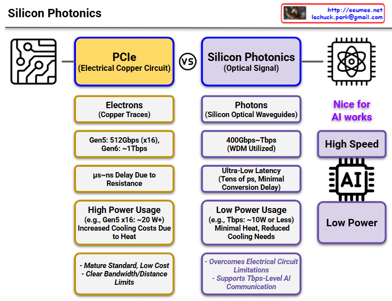
This diagram compares PCIe (Electrical Copper Circuit) and Silicon Photonics (Optical Signal) technologies.

PCIe (Left, Yellow Boxes)

  • Signal Transmission: Uses electrons (copper traces)
  • Speed: Gen5 512Gbps (x16), Gen6 ~1Tbps expected
  • Latency: μs~ns level delay due to resistance
  • Power Consumption: High (e.g., Gen5 x16 ~20W), increased cooling costs due to heat generation
  • Pros/Cons: Mature standard with low cost, but clear bandwidth/distance limitations

Silicon Photonics (Right, Purple Boxes)

  • Signal Transmission: Uses photons (silicon optical waveguides)
  • Speed: 400Gbps~7Tbps (utilizing WDM technology)
  • Latency: Ultra-low latency (tens of ps, minimal conversion delay)
  • Power Consumption: Low (e.g., 7Tbps ~10W or less), minimal heat with reduced cooling needs
  • Key Benefits:
    • Overcomes electrical circuit limitations
    • Supports 7Tbps-level AI communication
    • Optimized for AI workloads (high speed, low power)

Key Message

Silicon Photonics overcomes the limitations of existing PCIe technology (high power consumption, heat generation, speed limitations), making it a next-generation technology particularly well-suited for AI workloads requiring high-speed data processing.

With Claude

Transmission Rate vs Propagation Speed

Key Concepts

Transmission Rate

  • Amount of data processable per unit time (bps – bits per second)
  • “Processing speed” concept – how much data can be handled simultaneously
  • Low transmission rate causes Transmission Delay
  • “Link is full, cannot send data”

Propagation Speed

  • Speed of signal movement through physical media (m/s – meters per second)
  • “Travel speed” concept – how fast signals move
  • Slow propagation speed causes Propagation Delay
  • “Arrives late due to long distance”

Meaning of Delay

Two types of delays affect network performance through different principles. Transmission delay is packet size divided by transmission rate – the time to push data into the link. Propagation delay is distance divided by propagation speed – the time for signals to physically travel.

Two Directions of Technology Evolution

Bandwidth Expansion (More Data Bandwidth)

  • Improved data processing capability through transmission rate enhancement
  • Development of high-speed transmission technologies like optical fiber and 5G
  • No theoretical limits – continuous improvement possible

Path Optimization (More Fast, Less Delay)

  • Faster response times through propagation delay improvement
  • Physical distance reduction, edge computing, optimal routing
  • Fundamental physical limits exist: cannot exceed speed of light (c = 3×10⁸ m/s)
  • Actual media is slower due to refractive index (optical fiber: ~2×10⁸ m/s)

Network communication involves two distinct “speed” concepts: Transmission Rate (how much data can be processed per unit time in bps) and Propagation Speed (how fast signals physically travel in m/s). While transmission rate can be improved infinitely through technological advancement, propagation speed faces an absolute physical limit – the speed of light – creating fundamentally different approaches to network optimization. Understanding this distinction is crucial because transmission delays require bandwidth solutions, while propagation delays require path optimization within unchangeable physical constraints.

With Claude

Data Center

This image explains the fundamental concept and function of a data center:

  1. Left: “Data in a Building” – Illustrates a data center as a physical building that houses digital data (represented by binary code of 0s and 1s).
  2. Center: “Data Changes” – With the caption “By Energy,” showing how data is processed and transformed through the consumption of energy.
  3. Right: “Connect by Data” – Demonstrates how processed data from the data center connects to the outside world, particularly the internet, forming networks.

This diagram visualizes the essential definition of a data center – a physical building that stores data, consumes energy to process that data, and plays a crucial role in connecting this data to the external world through the internet.

With Claude

TCP Challenge ACK

This image explains the TCP Challenge ACK mechanism.

At the top, it shows a normal “TCP Connection Established” state. Below that, it illustrates two attack scenarios and the defense mechanism:

  1. First scenario: An attacker sends a SYN packet with SEQ(attack) value to an already connected session. The server responds with a TCP Challenge ACK.
  2. Second scenario: An attacker sends an RST packet with SEQ(attack) value. The server checks if the SEQ(attack) value is within the receive window size (RECV_WIN_SIZE):
    • If the value is inside the window (YES) – The session is reset.
    • If the value is outside the window (NO) – A TCP Challenge ACK is sent.

Additional information at the bottom includes:

  • The Challenge ACK is generated in the format seed ACK = SEQ(attack)+@
  • The net.ipv4.tcp_challenge_ack_limit setting indicates the limit number of TCP Challenge ACKs sent per second, which is used to block RST DDoS attacks.

Necessity and Effectiveness of TCP Challenge ACK:

TCP Challenge ACK is a critical mechanism for enhancing network security. Its necessity and effectiveness include:

  • Preventing Connection Hijacking: Detects and blocks attempts by attackers trying to hijack legitimate TCP connections.
  • Session Protection: Protects existing TCP sessions from RST/SYN packets with invalid sequence numbers.
  • Attack Validation: Verifies the authenticity of packets through Challenge ACKs, preventing connection termination by malicious packets.
  • DDoS Mitigation: Protects systems from RST flood attacks that maliciously terminate TCP connections.
  • Defense Against Blind Attacks: Increases the difficulty of blind attacks by requiring attackers to correctly guess the exact sequence numbers for successful attacks.

With Claude

TCP fast open

The image compares two TCP connection establishment methods:

  1. TCP 3-Way Handshaking (Traditional Method):
  • Shows a standard connection process with three steps:
    1. SYN (Synchronize) packet sent
    2. SYN + ACK (Synchronize + Acknowledge) packet returned
    3. ACK (Acknowledge) packet sent back
  • This happens every time a new TCP connection is established
  • Requires a full round-trip time (RTT) for connection setup
  1. TCP Fast Open:
  • Introduces a “Cookie” mechanism to optimize connection establishment
  • First connection follows the traditional 3-way handshake
  • Subsequent connections can use the stored cookie to reduce connection time
  • Benefits:
    • Reduces Round-Trip Time (1-RTT)
    • Better optimization for multiple connections
  • Requirements for TCP Fast Open:
    • Cookie security must be implemented
    • Both server and client must support the method
    • Intermediate network equipment must support the technique

The blue arrows in the TCP Fast Open diagram represent the cookie exchange and optimized connection process, highlighting the key difference from the traditional method.

With Claude

TCP/IP Better

This image is an informational diagram titled “TCP/IP and better” that explains various aspects of network protocols and optimizations.

The diagram is organized into three main sections:

  1. Connection
    • Shows “3 way Handshaking” with a visual representation of the SYN, SYN+ACK, ACK sequence
    • “Optimizing Handshake Latency” section mentions:
      • QUIC (Developed by Google, used in HTTP/3) → Supports 0-RTT handshake
      • TCP Fast Open (TFO) → Allows sending data with the first request using previous connection information
  2. Congestion Control
    • Lists “tahoe & reno” congestion control algorithms
    • Shows diagrams of Send Buffer Size with concepts like “Timeout 3-Dup-Ack” and “3-Dup Ack (Reno)”
    • “Minimizing Network Congestion & Fast Recovery” section mentions:
      • CUBIC → Less sensitive to RTT, enabling faster congestion recovery
      • BBR (Bottleneck Bandwidth and RTT) → Dynamically adjusts transmission rate based on real-time network conditions
  3. Header Remove
    • Shows TCP header structure diagram and “Optimize header” section
    • “Reducing Overhead” section mentions:
      • Compresses TCP headers in low-bandwidth networks (PPP, satellite links)
      • Uses UDP instead of TCP, eliminating the need for a TCP header

The diagram appears to be an educational resource about TCP/IP protocols and various optimizations that have been developed to improve network performance, particularly focused on connection establishment, congestion control, and overhead reduction.

With Claude

NAPI

This image shows a diagram of the Network New API (NAPI) introduced in Linux kernel 2.6. The diagram outlines the key components and concepts of NAPI with the following elements:

The diagram is organized into several sections:

  1. NAPI – The main concept is highlighted in a purple box
  2. Hybrid Mode – In a red box, showing the combination of interrupt and polling mechanisms
  3. Interrupt – In a green box, described as “to detect packet arrival”
  4. Polling – In a blue box, described as “to process packets in batches”

The Hybrid Mode section details four key features:

  1. <Interrupt> First – For initial packet detection
  2. <Polling> Mode – For interrupt mitigation
  3. Fast Packet Processing – For multi-packet processing in one time
  4. Load Balancing – For parallel processing with multiple cores

On the left, there’s a yellow box explaining “Optimizing interrupts during FAST Processing”

The bottom right contains additional information about prioritizing and efficiently allocating resources to process critical tasks quickly, accompanied by warning/hand and target icons.

The diagram illustrates how NAPI combines interrupt-driven and polling mechanisms to efficiently handle network packet processing in Linux.

With Claude