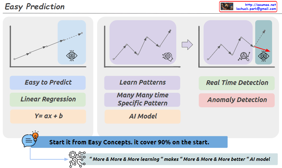
From Claude with some prompting
The image depicts the Autoregressive Integrated Moving Average (ARIMA) Integrated Moving Average Model, which is a time series forecasting technique.
The main components are:
- AR (Autoregressive):
- This component models the past pattern in the data.
- It performs regression analysis on the historical data.
- I (Integrated):
- This component handles the non-stationarity in the time series data.
- It applies differencing to make the data stationary.
- MA (Moving Average):
- This component uses the past error terms to calculate the current forecast.
- It applies a moving average to the error terms.
The flow of the model is as follows:
- Past Pattern: The historical data patterns are analyzed.
- Regression: The past patterns are used to perform regression analysis.
- Difference: The non-stationary data is made stationary through differencing.
- Applying Weights + Sliding Window: The regression analysis and differencing are combined, with a sliding window used to update the model.
- Prediction: The model generates forecasts based on the previous steps.
- Stabilization: The forecasts are stabilized and smoothed.
- Remove error: The model removes any remaining error from the forecasts, bringing them closer to the true average.
The diagram also includes visual representations of the forecast output, showing both upward and downward trends.
Overall, this ARIMA model integrates autoregressive, differencing, and moving average components to provide accurate time series forecasts while handling non-stationarity in the data.