From Claude with some prompting
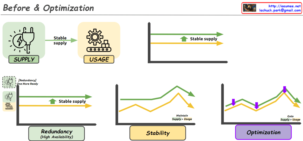
- “Just look (the average of usage)”:
- This stage shows a simplistic view of usage based on rough averages.
- The supply (green arrow) is generously provided based on this average usage.
- Actual fluctuations in usage are not considered at this point.
- “More Details of Usages”:
- Upon closer inspection, continuous variations in actual usage are discovered.
- The red dotted circle highlights these subtle fluctuations.
- At this stage, variability is recognized but not yet addressed.
- “Optimization”:
- After recognizing the variability, optimization is attempted based on peak usage.
- The dashed green arrow indicates the supply level set to meet maximum usage.
- Light green arrows show excess supply when actual usage is lower.
- “Changes of usage”:
- Over time, usage variability increases significantly.
- The red dotted circle emphasizes this increased volatility.
- “Unefficient”:
- This demonstrates how maintaining a constant supply based on peak usage becomes inefficient when faced with high variability.
- The orange shaded area visualizes the large gap between actual usage and supply, indicating the degree of inefficiency.
- “Optimization”:
- Finally, optimization is achieved through flexible supply that adapts to actual usage patterns.
- The green line closely matching the orange line (usage) shows supply being adjusted in real-time to match usage.
- This approach minimizes oversupply and efficiently responds to fluctuating demand.
This series illustrates the progression from a simplistic average-based view, through recognition of detailed usage patterns, to peak-based optimization, and finally to flexible supply optimization that matches real-time demand. It demonstrates the evolution towards a more efficient and responsive resource management approach.